CPU Profiling Basics: How to Locate Expensive Code Paths with Profiles

When an application feels slow, intuition is a poor debugger. Developers often guess at bottlenecks and optimize code that barely matters, while the real cost hides elsewhere. CPU profiling replaces guesswork with evidence by showing exactly where your program spends its processor time. Instead of measuring overall latency, a CPU profile breaks execution into functions and lines of code, revealing the expensive paths that dominate runtime. Learning to collect and interpret these profiles is a core skill for anyone responsible for software speed.

What CPU Profiling Actually Measures

A CPU profiler does not time every function with a stopwatch. Most modern profilers use sampling: many times per second, typically between 99 and 1000 Hz, the profiler pauses execution and records the current call stack. Over several seconds or minutes, these samples build a statistical picture of where time is spent. Functions that appear in many samples are responsible for more CPU time. This approach has very low overhead and works well for finding hot code, even in production systems.

It is important to distinguish CPU time from wall-clock time. A CPU profile only counts time when the thread is actively executing on a core. If your program is waiting for network I/O, disk, or a lock, that waiting will not show up as hot in a CPU profile. For those cases you need off-CPU or wall-clock profiling. Understanding this distinction prevents misinterpretation: a function that seems fast in a CPU profile might still be blocking progress elsewhere.

How to Read a CPU Profile to Find Slow Functions

Knowing how to read a CPU profile to find slow functions starts with understanding the three common views profilers provide: the flame graph, the call tree, and the top functions list. Each shows the same data from a different angle, and together they make expensive code paths obvious.

Start with the Big Picture: Flame Graphs

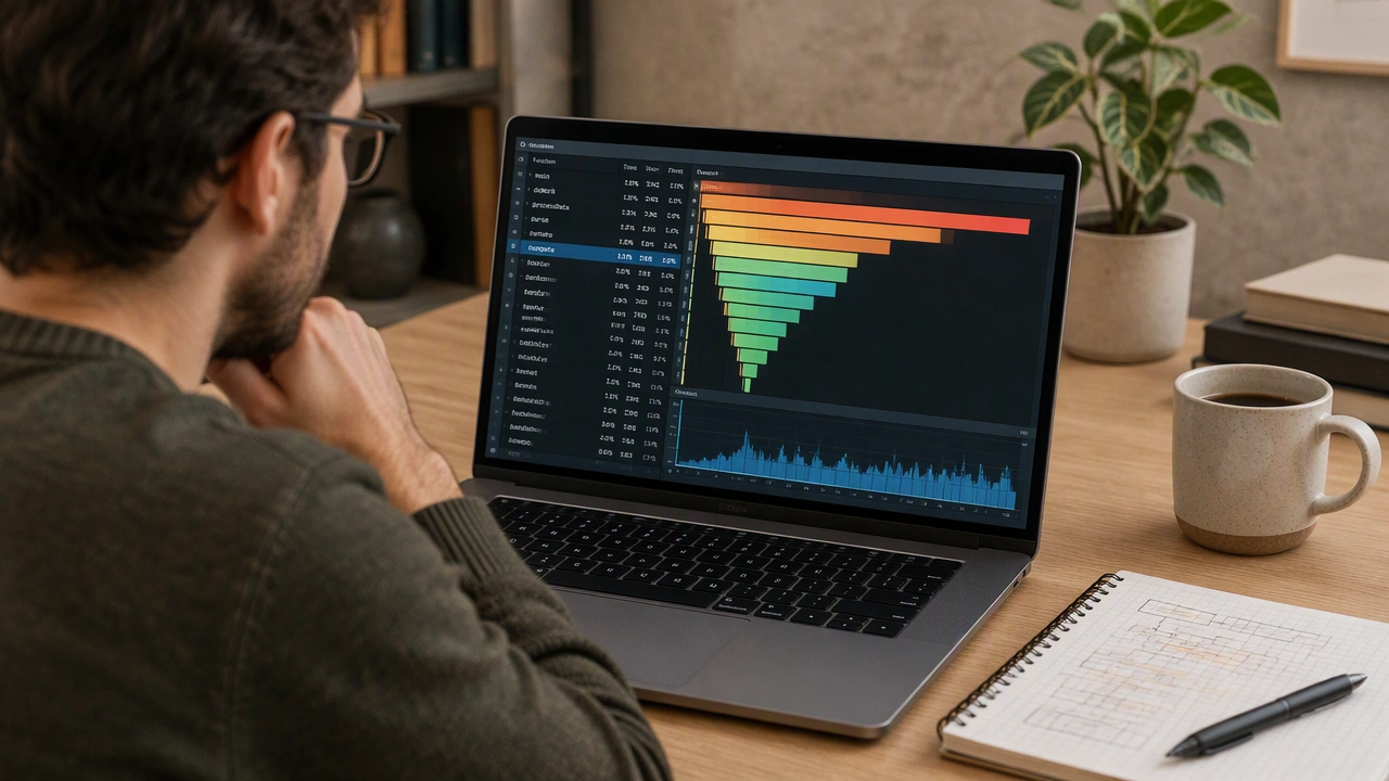
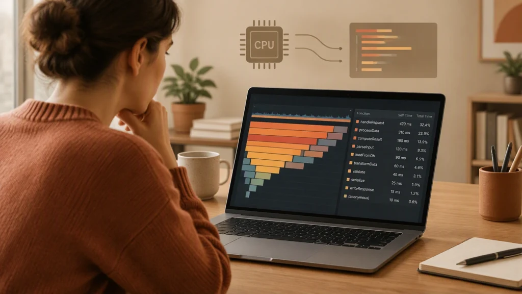
A flame graph visualizes all sampled stacks at once. The horizontal width represents the proportion of samples, which correlates with CPU time. The vertical axis shows stack depth, with the caller below and the callee above. To read it, look for wide plateaus near the top. A wide box means a single function was on-CPU for a large share of the profile. Click or hover to see the exact percentage and sample count. The widest towers usually point directly to your most expensive code paths, whether they are tight loops, heavy computations, or inefficient library calls.

Drill Down with Call Trees and Top-Down Views

While flame graphs are excellent for overview, a call tree gives you precise numbers and parent-child relationships. In a top-down tree, you start at the entry point, such as main or a request handler, and expand children sorted by total time. Total time includes time spent in the function and all functions it calls. Self time includes only time spent inside the function itself, excluding callees. If a function has high total time but low self time, the cost is in its descendants. If it has high self time, the function body itself is the bottleneck and deserves closer inspection.

Check the Numbers: Self Time vs Total Time

The list of top functions, often called hot spots or bottom-up view, ranks functions by self time regardless of who called them. This is the fastest way to answer what code is actually burning cycles. Sort by self time and look at the top five to ten entries. If you see the same function from multiple call paths, it is a shared hot spot. If you see unexpected functions, such as string formatting, regular expressions, or serialization, you have found accidental complexity. Always compare percentages to total samples to gauge impact. Optimizing a function that accounts for 1 percent of samples will not move the needle, while halving a 30 percent hot spot yields a visible speedup.

Common Patterns That Reveal Expensive Code Paths

After reviewing many profiles, certain shapes appear again and again. Recognizing them helps you move from observation to diagnosis without wasting time.

• Wide flat plateau: A single function dominating width at the top indicates a tight loop or heavy computation. Check for inefficient algorithms, such as O(n squared) loops, or repeated work that could be cached.
• Tall narrow tower: Deep stacks with small widths suggest excessive call depth or recursion. The cost may be call overhead or repeated setup and teardown in each layer.
• Repeated thin spikes of the same function: The same utility appears in many different branches. This points to a shared helper, like logging, allocation, or hashing, that is called too often.
• Unexpected library frames: Large blocks inside serialization, compression, or regex engines often mean you are formatting or parsing more than necessary.
• Kernel and garbage collection frames: Significant time in system calls or GC indicates allocation pressure, excessive I/O, or memory churn rather than application logic.

From Profile to Fix: Prioritizing What to Optimize

A profile tells you where time goes, but not every hot spot is worth fixing. Prioritize by impact and feasibility. Focus on code you control that appears near the top of the self-time list and is on the critical request path. Library and runtime costs are harder to change directly, but you can often reduce how often you call them.

• Measure before changing: Save the baseline profile and note total samples, request rate, and latency so you can compare after the fix.
• Fix the biggest self-time first: A 20 percent improvement on a 40 percent hot spot is more valuable than eliminating a 2 percent function entirely.
• Look for algorithmic wins: Replacing a quadratic loop, adding caching, or batching I/O often beats micro-optimizations.
• Verify with a second profile: After the change, collect a new profile under the same load to confirm the hot spot shrank and no new bottleneck appeared.

Profiling Tips for Accurate, Actionable Results

Good data makes interpretation easier. A noisy or biased profile can mislead you into optimizing the wrong path.

• Profile under realistic load: Use production-like traffic or representative benchmarks. Idle or synthetic workloads create artificial shapes.
• Collect long enough: Aim for at least 30 seconds to a few minutes to gather thousands of samples and smooth out variance.
• Keep symbols: Build with debug symbols or separate symbol files so function names are readable. Without symbols, you see only addresses.
• Compare profiles, not single numbers: Small changes in total time are noisy. Look for consistent shifts in flame graph width and top-function percentages.
• Profile again after deployment: Performance characteristics change with data size and user behavior. Regular profiling catches regressions early.

CPU profiling turns performance tuning from speculation into a repeatable workflow: collect samples, visualize stacks, identify the widest and hottest frames, and focus your effort where it matters most. With practice, reading a flame graph or call tree becomes quick and intuitive, letting you spot expensive code paths in seconds and guide optimizations that deliver real, measurable gains.